Visualizing Dominators
In this article we'll see two algorithms for computing dominators (the one actually gives us immediate dominators and sort of the dominator tree for free) with an emphasis on the intuition behind them through visualizations.
For the rest of this article I will assume that you at least have some familiarity with dominators in graph theory and control-flow graphs.
To refresh your knowledge, here's a classic example that showcases dominance relationships that is usually called a "diamond" (it's also the classic example when introducing phi nodes which are not much related to this article though).
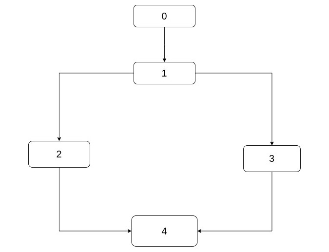
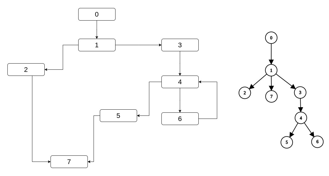
Let's say this is a part of a control-flow graph, the rectangles are the basic blocks and the flow goes from top (i.e. 0) to bottom (i.e. 4). This CFG could have been generated from this code for example:
void func(int n) {
  // Basic block 0 ...
  goto L1;
L1:
  // Basic Block 1 ...
  if (n < 0) {
    // Basic Block 2 ...
  } else {
    // Basic Block 3 ...
  }
  // Basic Block 4 ...
}
First of all note that the CFG I have drawn does not contain the code of basic blocks (which is also reflected in the code), only some way to identify them (in this case, integers). For the rest of this discussion we won't care about the code of the basic blocks, including blocks that contain conditional branches (like BB 1 here). While they obviously affect the control-flow, we don't know enough to use them in a static analysis (note that the compiler can deduce information about branches and e.g., convert a conditional branch to unconditional but this is a job of another part of the optimization pipeline - we're just given a CFG).
Second, unconditional branches like 0 -> 1 can't be naturally expressed in code hence the goto
but note that CFGs usually are made from a stricter form of intermediate representation that contains such branches (e.g. LLVM IR).
Anyway, back to the discussion about dominators, it should be clear here that 0 dominates 1, 2, 3, 4
and that 1 dominates 2, 3, 4. Also, pay attention that neither 2
nor 3 dominate 4. This is a subtle point when one first comes across dominators: There might
be a path from a node to another in which one seems to be "before" another
(like 2 here is before 4 in the source code). Bit if there are conditions involved for this path to be executed
then the former does not dominate the latter.
I should also note that while all 1, 2, 3, 4 are dominated by 0, only 1
has 0 as its immediate dominator. 2, 3, 4 respectively have 1
as their immediate dominator. And finally note that every node dominates itself by definition.
Ideally one should understand what is a dominator tree but I leave that for later. Before we move on, the final thing you should be comfortable with is the inclusion of an entry and exit node in CFGs. These are nodes that we insert to make our life (and algorithms) easier. For example, in the CFG above, basic block 0 did not exist initially (it even seems to be biased in the C code). But we inserted it and it is the entry node.
The same would be true for node 4 if
the ifs returned inside. What we want to achieve with these two blocks is to know that a function is always
entered in the same one block, the entry block, and is always exited in the same one block, the exit block.
For the rest of this article, the entry node will be assumed to be numbered 0 and the exit as the
CFG_size - 1. This assumption is held in the implementations as well.
The time has come to compute dominators for each node and before we go into the standard algorithms, you may want to pause and ponder how you could compute them yourself.
Our get-go algorithm is a naive implementation of the following data-flow framework.


You might be like as I was when I first saw this, specifically "Wait a second... I don't even understand a thing". Let's break it down.
The first equation is obvious: n0, which is the entry node, is only dominated by itself since
it doesn't have any predecessors anyway.
Then for all the rest of the nodes we see an equation that has to do with predecessors. At first glance, it makes sense that the dominators of a node will be somehow related to its predecessors since the latter are the ones that one must go through to reach the specific node.
In plain English it says: To find the dominators of a node, first put the node itself in the dominators set. Then, take all the common (i.e. intersection) dominators of its predecessors and put them in the set.
The simplest case of this equation is a linear graph (i.e. a graph where its node has one sucessor and one predecessor and every node points to its next except the exit). In this graph, a node's dominators are all its previous nodes. Applying the equation, every node has only one predecessor. We take the dominators of this predecessor (which are all its previous nodes plus itself) and we add it to the set.
The diamond case is where it gets interesting. Let's return back to the diamond CFG above. 4 has 2 predecessors,
2 and 3. Those have only one common dominator, 1,
which is the only dominator that ends up in 4's dominators after the intersection stage. This matches
our intuition because if a node has multiple predecessors, then none of these can dominate it because their paths to the node
are conditional. So, during the intersection stage, those will be cancelled out, leaving only the common ones.
One other way to think about this is to take the CFG from the node backwards and add to the dominators only the nodes at which the backward paths converge. Let's go back to the example.
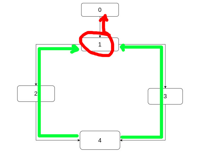
Starting from 4 and going backwards in the green paths, we see that these converge to 1.
Then you can also consider that they continue as a common red path.
This and similar observations are not just result of the dataflow equation but they may very well be the cause of it (we'll see a similar example later).
But then here comes another question which is: We don't necessarily know the dominators of the predecessors of a node, so what do we do then? Now we're going towards the algorithm.
One first observation is that we can go in depth-first-search, preorder-traversal. In literature you either see that as just depth-first search or reverse postorder traversal. Bottom line, we always visit the parents before the children, hence going down, we have the results we want. As it turns out, this is also more efficient and we'll see why.
But let's go back to the whatever order. One way to solve our problem is to start the dominator sets of each node (except the entry node) as being "all the nodes". Then, continuously remove from them until not set changes. This is a classic implementation of a fix-point algorithm, i.e. you just loop eternally until at some point there's no change. Of course you can't go willy-nilly with such algorithms, I mean we have to have previously proved that they actually actually end up in fixpoint otherwise we're going to loop forever.
We won't discuss its termination guarantee formally here but one way to persuade yourself that this procedure will eventually halt is that you continuously intersect sets without adding to them (note that the union with the node itself is not actual addition since it was there at the start). Which means that at some point, it's going to stop changing (in other words, the sizes of the sets is a monotonically decreasing function).
But what about its correctness? Going reverse postorder seems to be correct since we have the correct info about the predecessors and if that's true, then we saw how do we compute the dominators. To get some intuition as to why the whatever order will also yield correct results consider the case of a linear graph.
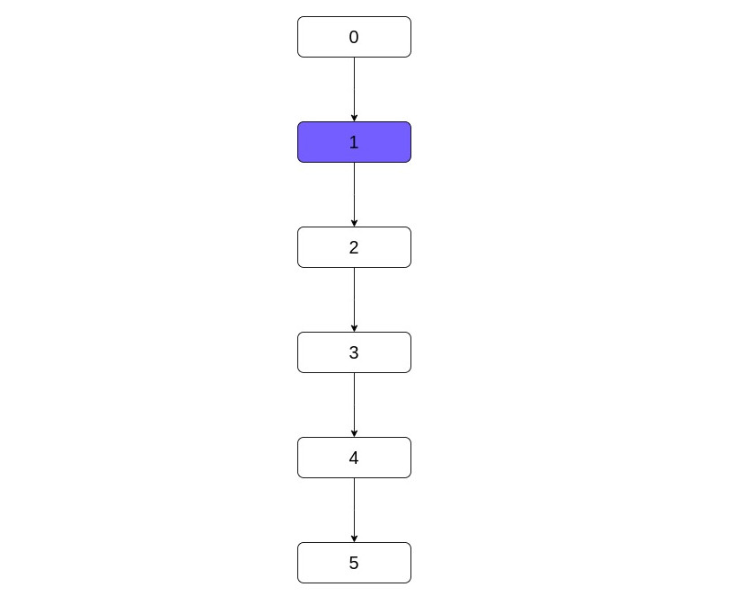
Consider the case of the reverse order, i.e. visiting nodes in the order: 5, 4, 3, 2, 1. The only
predecessor of 5 is 4 and its dominators are all the nodes (because of
the initialization referenced above). Because we have all the nodes, 5 gets all the nodes and no
change occurs. Fast-forward that for all the nodes except 1.
Its parent is the entry node and this is special. This was not initialized to "everything" but only to itself. Because of that,
1 also does not get everything but only the entry and itself. Which means, a change occurred
and we have to start over.
Here we see two important points. First of all, why the reverse postorder makes sense. Going into 1
and seeing the change I'm thinking "Great, go down now!! Pass the change on". But of course the algorithm doesn't quite
work like that, so we just loop again.
Then we see the central idea of fix-point algorithms. Changes might bring other changes, for example here we know that
1 will and should change the set of 2, so if we see a change,
we must loop again. Note that here we know that we have to go to 2 for the next change (e.g.
going to 1 again is useless), but in general we can't see the future so in the following iterations we don't do any specialized steps. We just do the same
steps over and over knowing that at some point this will end. And finally, exactly because we do the same
steps, if at some point no change occured then it won't ever occur.
An one sentence description of the algorithm is "Initialize the sets with all elements except the entry, then loop the equation until no change happens". And you get something like this:
compute_dominators(CFG cfg) {
  cfg[0].dominators = {0}
  for (bb in cfg except 0) {
    b.dominators = {all nodes in cfg}
  }

  do {
    change = false;
    for (bb in cfg except 0) {
      temp = {all nodes in cfg}
      for (pred in bb.predecessors) {
        temp = intersect(temp, pred.dominators)
      }
      temp = union(temp, {bb})
      if (temp != bb.dominators) {
        change = true
        bb.dominators = temp
      }
    }
  } while (change);
}
Formally this is not a general enough algorithm but that's not important here. We assume that we're given a CFG that can be indexed to get basic blocks. Basic blocks now contain at least an array of their predecessors and a set of their dominators (we fill the latter). Then the algorithm does what we have already discussed.
How do we implement that in practice? Well the only not obvious thing here is how do we implement the set. I chose to implement it using a bitvector. Every bit signifies if an element is in the set or not. Since the blocks are identified by integer numbers and because we want to keep in all elements in a range (i.e. [0..cfg_size - 1]), a bit vector is perfect. The intersection is only a logical OR between the bytes of two sets.
We can be a little more aggressive with performance. To start off, we can avoid multiple allocations of the temp set because
of course it's re-used. Not only that, but all the sets in the program have the same maximum number of elements so we can't ever be in a situation
where we can't fit the result of an intersection into it.
So we allocate it once with an invariant size and then re-use it. Also, note that initializing it, i.e. including all the elements, is
only a matter of lighting all bits on in the set. This is an operation that can be achieved with a memset
in the underlying bitvector, again making the two most used operations in this hot loop incredibly fast.
Finally, since the intersection is an OR, it should be able to be vectorized, not only by us, but also by the compiler. Furthermore, we can improve the algorithmic complexity by going through the basic blocks in reverse postorder as we said.
All these things result in an incredibly fast and simple implementation. Here's my implementation.
bitset.d contains code for the bitset while naive.d contains the main code. The code could
be smaller if you don't want to play with memory as much as I did (I allocate in a contiguous chunk the memory for the dominator sets and
also I use aligned memory for temp - these don't give big wins so you can skip them). The example graph is the one
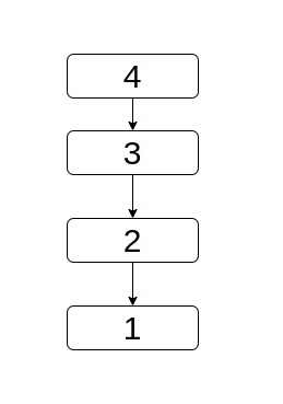
at the top of this page and it's an example from the book Advanced Compiler Design and Implementation.
Next I'm going to describe a presumably faster algorithm of great interest because of its simplicity and elegance. It is described in this paper: A Simple, Fast Dominance Algorithm.
The paper gives a good description but I'll try to give a different one, maybe less formal. So, remember what we said about traversing the CFG backwards until you find convergence? We'll take this idea one step ahead.
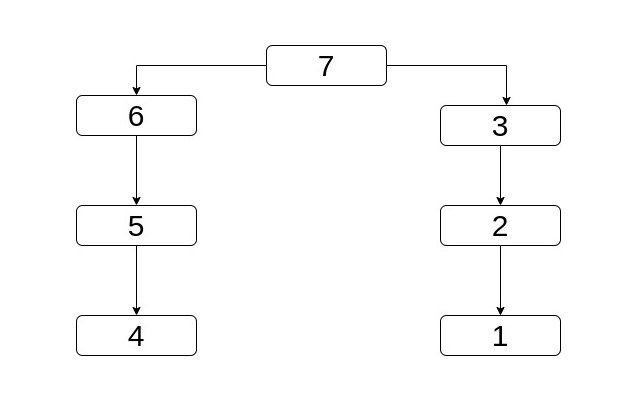
There's something called a dominator tree and this a tree in which every node has as its parent its (only one - except for entry) immediate dominator. Here are some examples:
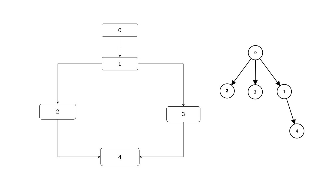
Let's imagine for a second that given a CFG, we're also given its dominator tree. If that happened first of all we would have a way to
find the immediate dominator of a node: Search for the node, take its parent. But also, if you remember in the preliminaries how we reasoned
that in this diamond (which is the first example above), 4 has two dominators except itself: 1, 0.
1 which is its immediate dominator and 0 which is the immediate dominator of its immediate dominator.
That is, a node's dominators are: The node, plus its immediate dominator, plus the immediate dominator of its immediate dominator etc. until we reach the entry.
This makes sense because as in the example, if to visit 4 you have to visit 1 and to
visit 1 you have to visit 0 then apparently to visit 4 you
have to visit 0.
Now, the way this relates to the dominator tree is that bottom line, to find the dominators of a node, you can take the path from the node to the entry, i.e. traverse the tree backwards (you can take the path any way you want but this backwards traversal is convenient in our case). So, we want a kind of alternate version of the dominator tree. We want a way to do fast search on the tree and also to be able to traverse it backwards.
Let's now go to the second important idea. Let's say we have a node and it has two predecessors. And we know the immediate dominator of each of these
two, can we find the immediate dominator of the node ? We have already come across this intuitively. Remember in the diamond example that
4 has two predecessors, 2, 3. We said that in the end 4
has 1 as its immediate dominator because 1 is where 2, 3
meet if we take paths backwards in the CFG. Let's see a more complicated example where the two predecessors of a node don't have the same
common predecessor (and immediate dominator).
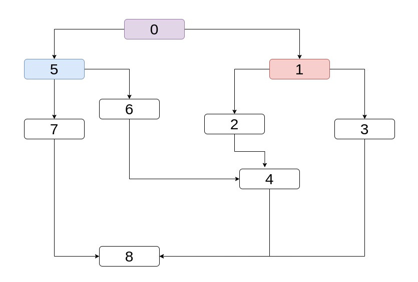
Take node 4. That has two predecessors, 2, 6. We know the immediate dominator of
both, it is 1 and 5 respectively. What is the immediate dominator of 4 ?
It is 0. It's always the "most immediate" dominator of the two predecessors at hand. Because it's like asking "What is
the closest node that I will have to take no matter what to reach any of these predecessors". This is
where it comes the idea of going backwards and seeing where the paths merge.
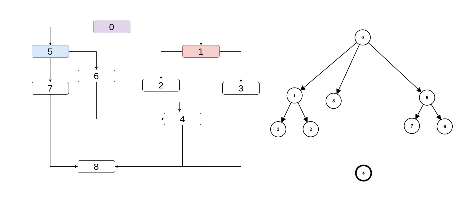
But also, the "most immediate" dominator is clearer if we have the dominator tree. It's the lowest common ancestor (i.e. the "lowest" node at the
tree that is ancestor of both) and intuitevely it is exaclty what we want. Take a look at "semi-complete" the dominator tree of the CFG above, without
4 having any parent (after all, this is what we're trying to find). Note that the lowest common ancestor of
1, 5 is 0.
An even more interesting example is if we have partial dominance info about the predecessors of 8.
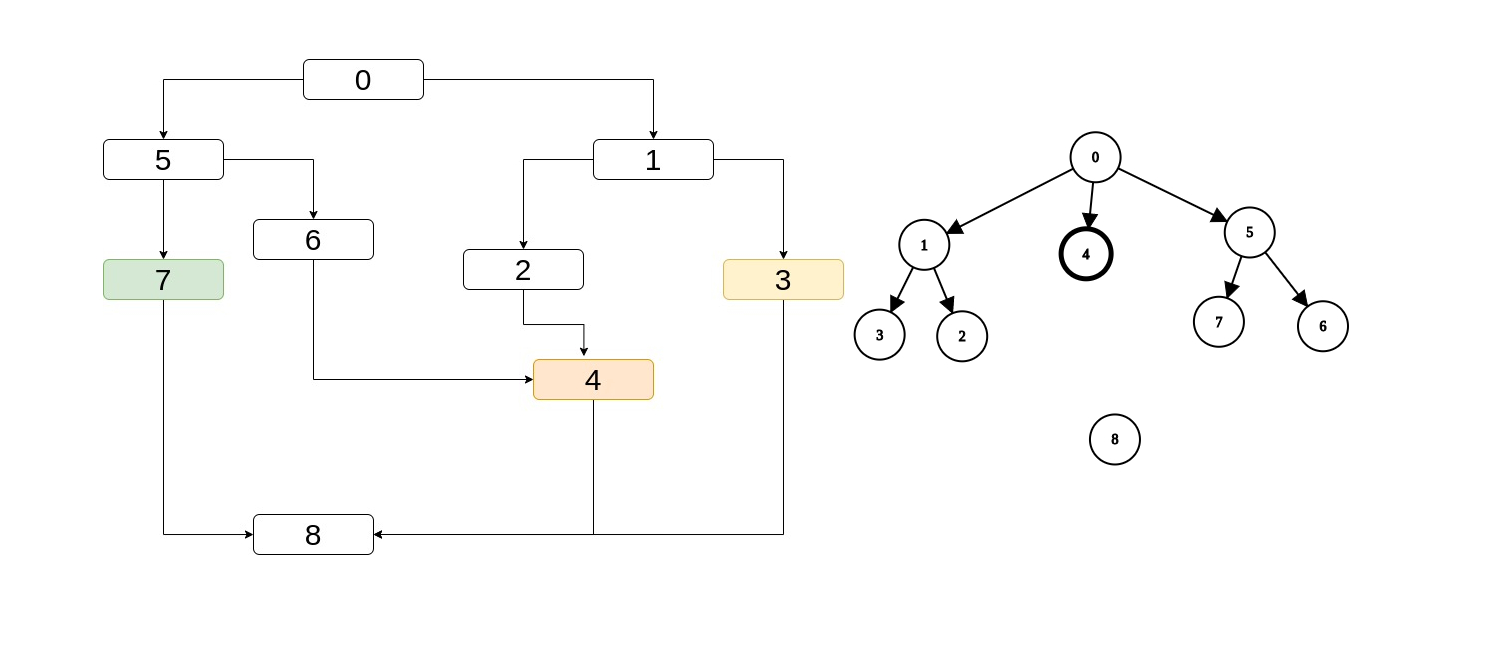
It has 3 predecessors colored in the drawing whose lowest common ancestor is again 0.
Now, let's go to the algorithmic part. The idea is that we'll represent the dominator tree in a way that suits our needs. It will be an array that contains for each basic block its immediate predecessor. Note that in that way, we accomplish the two things we want: We can both index the tree fast and we can traverse it backwards (e.g. take the immediate dominator of a basic block then index again the array to find its immediate dominator).
Instead of this tree being given, we will build it iteratively (actually the whole point of this algorithm is to build this array - then as we said, if we have it, we can find dominators implicitly). And to build it, we'll use the reasoning above, i.e. knowing the immediate dominator of two predecessors of a basic block, how do we find this block's immediate dominator -> by traversing the tree backwards until we converge.
Before I present the algorithm, how do we actually find this lowest common ancestor ? Let's say we have two nodes a, b
in the tree and we want to find their lowest common ancestor. If a is higher in the tree (more towards the root / entry)
than b, then we have to move b higher and vice versa. We do that until the two meet
(and they will meet even if that means at the entry because it is a tree not a forest). In the example with 8 above,
let's assume the two predecessors we're working with are 7, 3. Their immediate dominators are 5, 1
respectively and we want to find their lowest common ancestor. 5, 1 are in the same height so we can move one arbitrarily.
Let's say we move 5. Then, we'll see that now 5 became 0 and
0 is higher than 1 in the tree, so we have to move 1.
And now they met. So 8's immediate dominator is 0 and we note it in the array.
So, now remember we don't have the tree, we have only an array. We know how to "move up" but we don't know how to answer the question "is this
higher than the other ?". For that reason, we'll compute the postorder traversal (in which remember, nodes at the top of the CFG have higher
numbers because they're visited later) of the CFG (which we need anyway, as we'll see below). Note that if a < b
in the postorder traversal, then the first case is that they are in the same sub-tree, in which case
b is higher by definition (of postorder) and thus we have to move a up. Take a look
in the linear graph below in which nodes have been labeled with their postorder visit time.
In the other case they're in different sub-trees and in this case we have to move both. But we'll choose to move a here too for uniformity. Eventually, we'll move it to their lowest common ancestor which is definitely higher than both in which case we'll start to move
b up and eventually reach it. Take a look at the example below at which nodes again are labeled with their
postorder traversal.
Here 3 < 4 but obviously 3 is higher in dominator tree (which interestingly, is the CFG
itself in this case). However it doesn't matter because we're going to move it to 7 at which point
we'll start moving 4 up.
So that's it, we covered all the necessary theoretical background and it's time to code. Here's the C / D code of the main algorithm which is so simple that it is better than pseudocode (here's an actual implementation in C).
void compute_dominators(CFG cfg) {
  // Some initialization steps and e.g. get postorder.

  // Map its basic block to its postorder traversal.
  foreach (p ; postorder) {
    postorder_map[p] = counter;
    ++counter;
  }

  bool change;
  do {
    change = false;
    foreach_reverse (int i; postorder) {
      BasicBlock *bb = &cfg[i];
      int new_idom = bb.preds[0];  // Arbitrarily choose the first predecessor
      foreach (pred ; bb.preds[1..bb.preds.length]) {
        if (cfg.idoms[pred] != CFG.UNDEFINED_IDOM) {
          new_idom = intersect(new_idom, pred, cfg.idoms, postorder_map);
        }
      }
      if (cfg.idoms[i] != new_idom) {
        cfg.idoms[i] = new_idom;
        change = true;
      }
    }
  } while (change);
}

int intersect(int b1, int b2, Array!int idoms, Array!int postorder_map) {
  while (b1 != b2) {
    if (postorder_map[b1] < postorder_map[b2]) {
      b1 = idoms[b1];
    } else {
      b2 = idoms[b2];
    }
  }
  return b1;
}
Our task is to fill cfg.idoms. We compute the postorder traversal and map it to each node because we'll need to know
it as we said. Then, the loop does something very simple. It applies what we said to find the immediate dominator of a node given the immediate
dominators of its predecessors, but it does it in pairs of 2. For example, if the node has two predecessors, it will set new_idom
to the first and for the second it'll find the lowest common ancestor using intersect(). If it has more, it will do
the same for the other predecessors, every time using the one-just-found (new_idom) one as the first predecessor and the new one (pred) as the second.
One final note is that here going in reverse postorder traversal is not optional! In intersect() we're indexing the
immediate dominators of nodes and if one such ends up being undefined, which in this case is -1, we'll then index
beyond the bounds of the array (because -1 will be less than any basic block). Going reverse postorder we guarantee that the tree is built
from top to bottom and info about predecessors is always available.
Maybe to your surprise, my (not deeply thought) benchmarks showed that the naive algorithm is about 10x faster! The algorithm may seem faster but in practice it doesn't make sense to be, at least to me. The naive algorithm uses the hardware amazingly well. It's taking full advantage of cache locality (everywhere contiguous memory and the operations are linear and predictable), it has no mispredicted branches, no excessive memory allocations, and of course it takes full advantage of SIMD units. I mean now that I'm thinking about it, it doesn't even enforce a specific order so for some graphs, it may make sense to do it multi-threaded.
On the other hand, while the last algorithm is memory efficient (although I don't if it's more than the naive in practice) and it also seems to be hardware-aware, because we're traversing a "tree" but we don't chase pointers; it is actually serialized. The problem is that the accesses on this tree are "random" (random enough to not benefit cache-line (pre)fetching). There may be a better, postorder-based heuristic way to order the basic blocks in the array but as it is now, things are not going too well. Definitely though it's a very impressive algorithm and I may very well be missing some implementation details that would make it faster. Unfortunately, the implementation used in the paper is not available as far as I know.
I have not yet found time to complete a good explanation on this algorithm. However, I have created this video, which I hope will help you understand a particularly subtle point in the algorithm.