The Cryptic Proof of Semidominators in the Lengauer-Tarjan Algorithm
Dominance is one of the most ubiquitous concepts in compilers. By far the most popular algorithm for discovering dominance relationships is the Lengauer-Tarjan algorithm - a fascinating but scary piece of genius. In this article, we will deconstruct its most important part, the computation of semidominators. To tackle it, I'll use a lot of intuition, crappy drawings and some imagination.
Dominance is no joke in compiler optimization. We discover loops based on it, we build SSA based on it, we find control dependences based on it. The applications are just countless.
The Lengauer-Tarjan algorithm is no joke either. It is used, or was used, in basically every optimizing compiler ever. LLVM used to use it, the Go compiler still uses it, and the same is true for GCC.
So, every compiler optimization person is supposed to know this beast. But if you're like me, the first (or second, or third...) time you read the paper, you were like "what theeee....". It's not exactly obvious why it works (although it's fairly easy to implement).
In this article, I will try to decrypt its most important part – the computation of semi-dominators. If you nail it, you will be equipped to tackle the rest of the algorithm.
The good and surprising news is that you literally need to know nothing about compiler optimization. The content falls under algorithms and graph theory and just happens to be useful to compiler people. But, some knowledge on those two areas is beneficial to be able to follow the article. If you know what the following terms are, you're good to go: control-flow graph, dominance, dominator tree and depth-first-search (DFS). If you're also a little familiar with the paper, even better. For instance, you might want to remind yourself what is a semidominator. And it might be a good idea to take a look at (the short) Appendix A.
We'll start with a central point throughout the algorithm, which is the depth-first search (DFS) on the control-flow graph (CFG). A DFS visits all the vertices using a subset of the edges of the CFG, and this combination of this subset of edges with the vertices makes up a tree - the DFS tree. You can see an example CFG below, with a DFS animated.
The blue edges are not new edges. They are the subset of the (red) edges of the CFG that we use during the DFS. These blue edges along with all the nodes make up the DFS tree (basically, the DFS tree is a sub-graph of the CFG).
We stub the vertices with incrementing
numbers, which you can think as the visit time; the higher the number, the later
we visited a node during the DFS. This means that if a node v has a
smaller DFS number than a node w, then it means we visited v before
w during the DFS.
A related point is that if v is an ancestor of w in the DFS tree (i.e.,
there is a path from v to w in the DFS tree), then necessarily
v has a smaller DFS number than w. This is because we must
have visited the ancestor first, in order to discover a DFS-tree-path to the node. In the graph above,
A is an ancestor of B and E and so, it has a smaller
DFS number than both of them.
However, the inverse is not true! That is, if v has a smaller DFS
number than w, then it is not necessarily the case that v is an
ancestor of w. In the graph above, B has a smaller DFS number
than E, but it is not its ancestor.
Such kinds of discussions about ancestors and numbers in the DFS tree are going to come up a lot, so for brevity, when I say "ancestor", I will mean "ancestor in the DFS tree" and when I say "A is smaller than B", I will mean "node A has a smaller DFS number than node B".
While we're on the topic of clarifying things, note the difference between CFG and DFS-tree paths. A DFS-tree path is always a CFG path (since the DFS tree is a sub-graph of the CFG), but the inverse is not necessarily true. When I say "path", I will mean CFG-path. When I want to talk specifically about tree paths, I will clarify it.
I should note that there can be more than one DFS's that we can do on the same graph. For instance,
in the graph above, when we visited node A, we then visited B,
but we could have just as well visited E instead. A subtle corollary is that a node
v can be an ancestor of a node w in one DFS but not in another. For instance,
from R, we first took the edge to A, which made A an
ancestor of B. But we could have first taken the edge to B, in which
case A would be the last node we visit and it would not be an ancestor of B.
The important thing is that no matter the DFS, the proof does not change (this probably requires a proof that I'll skip for now). However, for your own convenience, it's a good idea to stick with some convention regarding how you visit edges, both when you draw in paper but maybe most importantly, when you code it. It's going to help in reproducing intermediate states when you're debugging.
So, we know the following, which we'll refer to as Equation (1) or just (1) (as in the paper):
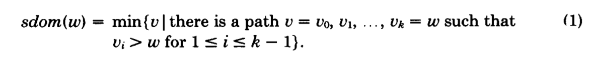
Note that the above is a definition. We know it! What it defines
is that the semidominator of w is a node, it has a
CFG-path to w, and everything on this path except the starting node
and w
is bigger than w. The semidominator is the minimum
node with this property.
Note that from the definition, it might seem that the semidominator
itself might be bigger than w, but this is impossible.
Because of Lemma 3 in the paper, sdom(w) is an ancestor of w
which means that it is also smaller.
Having this definition, we want to prove the following theorem:
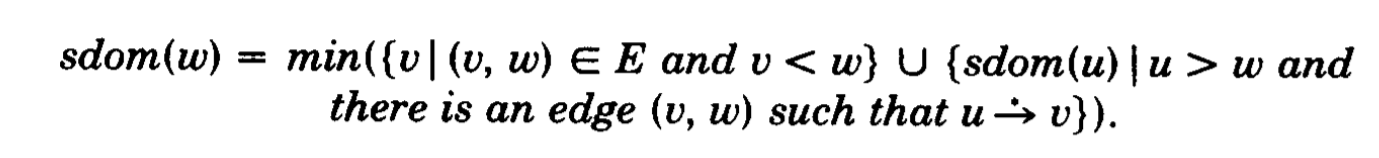
The proof is structured nicely, as it is split in two similar and complementary parts, each of which
has two sub-parts. To prove the theorem, we need to prove that sdom(w) = x,
where x is the right-hand side in the picture above (i.e., the theorem). Note here that x is a node.
One common way to approach such a proof, where we want to prove that two things are equal and we can't prove it directly, is to first prove that the one thing is smaller or equal to the other. Then, prove that it is bigger or equal to the other. The combination implies that the two things are equal.
This is what we will do here. We will first prove that sdom(w) <= x and then
that sdom(w) >= x. These are the two parts of the proof. Each part
has two subparts. If you pay attention to x, it is basically a minimum on a union. The two
sub-parts deal with the two sides of the union separately.
sdom(w) <= x
First, we consider the case where x has a single edge to w,
and it is smaller than w i.e., we consider the left-hand side of the union (of x). This case is
trivial because the definition of semidominators (i.e., (1)) considers paths of which
the (single-edge) path we're talking about is a subset. Since (1) takes the minimum
of all the paths it considers, sdom(w) must be smaller than x.
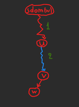
The other sub-part is more interesting and it is the right-hand
side of the union in x. It looks like this:
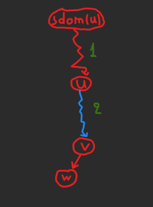
The squiggly arrows denote paths and not edges. We have two such paths, numbered (with green) 1) and 2).
On the other hand, the arrow from v to w is a single edge. Also, red
arrows denote arbitrary paths/edges, while the blue arrow denotes a DFS-tree path.
So, the right-hand side of the union, and the picture above, describe the following. There is a node u, which is bigger than
w, and that is an ancestor of some
node v (and thus there is a tree path from u to v).
v in turn has an edge to w. Now, u has a
semidominator sdom(u), and that is our x. What we want to show is that this whole path
sdom(u) -> ... -> u -> ... -> v -> w makes sdom(u) (i.e., x in this case) a candidate for a semidominator of w.
I will use the informal term "candidate" a couple of times in the article, so let me explain it.
As you may have guessed, we will deal with a lot of minimums throughout the proof. All the minimums
follow a particular pattern: Take the minimum of some set (of nodes), whose elements satisfy some
constraints; call them C. When referring to some minimum, I will call a "candidate"
for this minimum a node that satisfies C. In this case, we are talking
about the minimum appearing in (1). So, a candidate for this minimum is a node
that appears at the beginning of a path that ends in w, and in which path all the nodes,
except the beginning and the end, are bigger than this w.
Now, we want to show that sdom(u) is a candidate for the semidominator of w.
It is indeed and we can break the path in 5 pieces to see that: sdom(u),
path 1), u, path 2), v. First, by assumption, u > w.
Then, by the definition of the semidominator, everything in path 1)
is bigger than u and so bigger than w. Then, everything in path
2) (except u but including v) is also bigger than u and so, bigger than w, because u is an ancestor of every node in this
path (because 2) is a tree path). Thus, we proved that everything in the path
sdom(u) -> ... -> u -> ... v -> w above
is bigger than w, except possibly sdom(u).
So, sdom(u) (or x here) is a candidate and because sdom(w)
is the minimum of all the candidates, sdom(w) <= x.
sdom(w) >= x
In the Part 1, the approach looked like this: Take a case on x (first the left,
then the right-hand side of the union) and then show that this case is a subset of those
considered in (1). Because (1) takes a minimum, sdom(w) <= x. Now, we will
do the opposite. We will take two cases on the sdom(w) and for each
case, we will show that each falls under a side of the union in
x (i.e., it is a candidate of x).
Because x takes the minimum of all its candidates,sdom(w) >= x.
So, first, we will take the case where sdom(w) has a single edge to w.
By Lemma 3, i.e., that sdom(w) is an ancestor of w, it follows
that sdom(w) < w (see the warm-up). These two properties make sdom(w) a
candidate of the left-hand side of the union of x (i.e., sdom(w)
is union's v) and thus, sdom(w) >= x in this case.
Now, let's go to the second case. Here, sdom(w) is connected
with a multi-edge path P to w. This path
looks like sdom(w) -> ... -> w, with everything in this path
except the beginning and the end being bigger than w (by assumption; this
is a case of sdom(w)). Remember,
what we ultimately want to show is that sdom(w) is a candidate of x. To
do that, we need to find a "v" and a "u" (possibly on P)
that act like the v and u of the right-hand side of x.
That means 3 things: (a) u > w, (b) u is an ancestor of v
and (c) v has an edge to w. If we do that, then sdom(u)
is a candidate of the right-hand side of the union, and thus sdom(u) >= x.
That doesn't end the proof because we still haven't involved sdom(w) anywhere;
remember that ultimately we want to prove that sdom(w) is a candidate.
To involve it, we will show that sdom(w) >= sdom(u) and because sdom(u) >= x,
that proves what we want. But how will we do all that? The summary is that we will find
v and u on P, and that will help us mix all of the:
sdom(u), sdom(w) and x.
We'll start by finding a v, which is easy. We pick the the next
to the last node in P, where
the last is w. In other words, P looks like this:
sdom(w) -> ... -> v -> w, that is, v is the node that connects
the rest of the path with w. Note that there exists such a v
which is not sdom(w) and the reason is that this path has more than one edge
(otherwise, we would be in the first sub-part of Part 2, which we already considered).
Now, we need to find a suitable u. We will pick the closest-to-sdom(w) node in the path such that u is an ancestor of v; but it should not be sdom(w). Such a u exists because v is a candidate for
a u (and any node is an ancestor of itself). Note that right off the bat, we
know that u > w as everything in (the "middle" of) P,
including u, is bigger than w by assumption. Also, because of the
way we defined u, it is an ancestor of v and also by its definition,
v has an edge to w.
The picture looks as follows, which non-coincidentally, might remind you of the picture
we saw in Part 1. The difference is that sdom(u) has been replaced by
sdom(w)
Ok, now remember, we need to show 2 things: sdom(u) >= x and sdom(w) >= sdom(u). The former is trivial. Because of the way that we have picked v and u,
sdom(u) is a candidate of the right-hand side of x. The latter
is more involved. We will show that everything in path 1) (in the picture above) is bigger than
u. If that is the case, then sdom(w) is a candidate for being
the sdom(u). Because sdom(u) is the minimum of all the candidates (remember
the definition (1) of a semidominator), sdom(w) >= sdom(u).
So, let's get right to it. It's a proof by contradiction, so, suppose there's a node z
in path 1), such that z < u (note that it can't be equal to u because
the DFS numbers are unique and so only u is equal to u). If there are multiple choices for z, choose
the one that is closest to sdom(w) (but not sdom(w)). Because z < u, it means
that we visited z before u. And because there is a path from z
to u, it means that in the DFS we can reach u from z.
Because we visited z first, it means that the first time we reached/visited
u during the DFS, was through a tree path from z. That in turn
makes z an ancestor of u. But note that u is
an ancestor of v, but not just any ancestor. It is the closest-to-sdom(w) ancestor by assumption. However, if z is an ancestor of u,
then z is also an ancestor of v. But z is closer to sdom(w)than u. This invalidates the assumption that u is the closest
and hence, we end up in a contradiction.
This is a sick algorithm and hopefully my explanation met high standards. If dominance algorithms sound interesting, here's an article visualizing another two: Visualizing Dominators. You might also want to check more articles by clicking "Go to Home" on the bottom-right corner.